===== Matching Polytopes =====
In this tutorial we will use ''%%polymake%%'' to construct and analyse matching polytopes.
First we construct a graph, the complete graph on four nodes:
> $K4=new GraphAdjacency(4);
> for (my $i=0; $i<4; ++$i) {
>   for (my $j=$i+1; $j<4; ++$j) {
>     $K4->edge($i,$j);
>   }
> }
(See also the [[apps_graph|Tutorial on Graphs]] for more on the construction of graphs.)
Next we like to have the node-edge-incidence matrix of our graph. Since the latest release of ''%%polymake%%'' does not yet support this, we have to write the function ourselves:
> sub node_edge_incidences {
>     my $g=shift;
>    my $A=new Matrix($g->nodes, $g->edges);
>     my $k=0;
>    for (my $i=0; $i<$g->nodes-1; ++$i) {
>        foreach (@{$g->adjacent_nodes($i)}) {
>            if ($_>$i) {
>                $A->[$i]->[$k]=1;
>                $A->[$_]->[$k]=1;
>                ++$k;
>            }
>        }
>    }
>    return $A;
> }
Now we can construct the node-edge-incidence matrix of our graph ''%%K4%%'':
> $A=node_edge_incidences($K4);
> print $A;
1 1 1 0 0 0
1 0 0 1 1 0
0 1 0 1 0 1
0 0 1 0 1 1
With this we can now construct the constraint matrix consisting of an upper part for the nonnegativity constraints $x_e \ge 0$ ...
> $I=new Matrix([[1,0,0,0,0,0],[0,1,0,0,0,0],[0,0,1,0,0,0],[0,0,0,1,0,0],[0,0,0,0,1,0],[0,0,0,0,0,1]]);
> $Block1=new Matrix(new Vector([0,0,0,0,0,0]) | $I);
... and a lower part for the constraints $\Sigma_e x_e \le 1$ for each vertex $v \in V$, where the sum is over all edges e containing v:
> $Block2=new Matrix(new Vector([1,1,1,1]) | -$A);
Now we can put both parts together and define the polytope:
> $Ineqs=new Matrix($Block1 / $Block2);
> $P=new Polytope(INEQUALITIES=>$Ineqs);
The matching polytope of ''%%K4%%'' is the integer hull of ''%%P%%'':
> $P_I=new Polytope(POINTS=>$P->LATTICE_POINTS);
We can analyse some elementary properties of ''%%P_I%%'' ...
> print $P_I->POINTS;
1 0 0 0 0 0 0
1 0 0 0 0 0 1
1 0 0 0 0 1 0
1 0 0 0 1 0 0
1 0 0 1 0 0 0
1 0 0 1 1 0 0
1 0 1 0 0 0 0
1 0 1 0 0 1 0
1 1 0 0 0 0 0
1 1 0 0 0 0 1
> print $P_I->FACETS;
0 0 0 0 0 0 1
0 0 0 0 0 1 0
1 -1 -1 -1 0 0 0
1 -1 -1 0 -1 0 0
0 0 0 0 1 0 0
0 0 0 1 0 0 0
0 0 1 0 0 0 0
1 -1 0 -1 0 -1 0
1 -1 0 0 -1 -1 0
1 0 0 -1 0 -1 -1
1 0 0 0 -1 -1 -1
0 1 0 0 0 0 0
1 0 -1 -1 0 0 -1
1 0 -1 0 -1 0 -1
> print $P_I->N_FACETS;
14
... and compare them with the according properties of the defining polytope ''%%P%%'':
> print $P->VERTICES;
1 0 0 1 1 0 0
1 1 0 0 0 0 1
1 0 0 0 1/2 1/2 1/2
1 0 0 0 0 0 1
1 0 1/2 1/2 0 0 1/2
1 0 0 1 0 0 0
1 1/2 1/2 0 1/2 0 0
1 0 0 0 1 0 0
1 0 1 0 0 0 0
1 1 0 0 0 0 0
1 0 0 0 0 0 0
1 0 1 0 0 1 0
1 0 0 0 0 1 0
1 1/2 0 1/2 0 1/2 0
> print $P->VOLUME;
1/72
> print $P_I->VOLUME;
1/90
Next we analyse the combinatorics of ''%%P_I%%'': 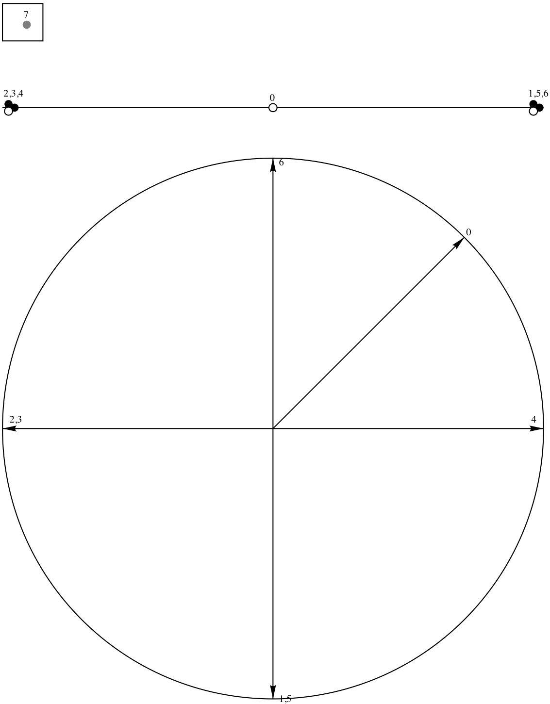
> print $P_I->AMBIENT_DIM, " ", $P_I->DIM;
6 6
> print $P_I->F_VECTOR;
10 39 78 86 51 14
> print $P_I->FACET_SIZES;
8 8 6 6 8 8 8 6 6 6 6 8 6 6
> $facet0=facet($P_I,0);
> print $facet0->AMBIENT_DIM, " ", $facet0->DIM;
6 5
> print rows_labeled($facet0->VERTICES_IN_FACETS);
0:0 2 3 4 5 7
1:3 4 5 6 7
2:2 4 5 6 7
3:0 1 3 5 6 7
4:0 1 2 5 6 7
5:0 1 2 3 4 7
6:1 3 4 6 7
7:1 2 4 6 7
8:0 1 2 3 4 5 6
> $facet0->GALE;
The Gale diagram of ''%%facet0%%'' is depicted on the right.