This tutorial is probably also available as a Jupyter notebook in the demo folder in the polymake source and on github.
Different versions of this tutorial: latest release, release 4.13, release 4.12, release 4.11, release 4.10, release 4.9, release 4.8, release 4.7, release 4.6, release 4.5, release 4.4, release 4.3, release 4.2, release 4.1, release 4.0, release 3.6, nightly master
Matching Polytopes
In this tutorial we will use polymake to construct and analyse matching polytopes.
First we construct a graph, the complete graph on four nodes:
> $K4=new GraphAdjacency(4);
> for (my $i=0; $i<4; ++$i) {
>   for (my $j=$i+1; $j<4; ++$j) {
>     $K4->edge($i,$j);
>   }
> }
(See also the Tutorial on Graphs for more on the construction of graphs.)
Next we like to have the node-edge-incidence matrix of our graph. Since the latest release of polymake does not yet support this, we have to write the function ourselves:
> sub node_edge_incidences {
>     my $g=shift;
>    my $A=new Matrix<Int>($g->nodes, $g->edges);
>     my $k=0;
>    for (my $i=0; $i<$g->nodes-1; ++$i) {
>        foreach (@{$g->adjacent_nodes($i)}) {
>            if ($_>$i) {
>                $A->[$i]->[$k]=1;
>                $A->[$_]->[$k]=1;
>                ++$k;
>            }
>        }
>    }
>    return $A;
> }
Now we can construct the node-edge-incidence matrix of our graph K4:
> $A=node_edge_incidences($K4);
> print $A;
1 1 1 0 0 0
1 0 0 1 1 0
0 1 0 1 0 1
0 0 1 0 1 1
With this we can now construct the constraint matrix consisting of an upper part for the nonnegativity constraints $x_e \ge 0$ …
> $I=new Matrix<Int>([[1,0,0,0,0,0],[0,1,0,0,0,0],[0,0,1,0,0,0],[0,0,0,1,0,0],[0,0,0,0,1,0],[0,0,0,0,0,1]]);
> $Block1=new Matrix<Int>(new Vector<Int>([0,0,0,0,0,0]) | $I);
… and a lower part for the constraints $\Sigma_e x_e \le 1$ for each vertex $v \in V$, where the sum is over all edges e containing v:
> $Block2=new Matrix<Int>(new Vector<Int>([1,1,1,1]) | -$A);
Now we can put both parts together and define the polytope:
> $Ineqs=new Matrix<Rational>($Block1 / $Block2);
> $P=new Polytope<Rational>(INEQUALITIES=>$Ineqs);
The matching polytope of K4 is the integer hull of P:
> $P_I=new Polytope<Rational>(POINTS=>$P->LATTICE_POINTS);
We can analyse some elementary properties of P_I …
> print $P_I->POINTS;
1 0 0 0 0 0 0
1 0 0 0 0 0 1
1 0 0 0 0 1 0
1 0 0 0 1 0 0
1 0 0 1 0 0 0
1 0 0 1 1 0 0
1 0 1 0 0 0 0
1 0 1 0 0 1 0
1 1 0 0 0 0 0
1 1 0 0 0 0 1
> print $P_I->FACETS;
0 0 0 0 0 0 1
0 0 0 0 0 1 0
1 -1 -1 -1 0 0 0
1 -1 -1 0 -1 0 0
0 0 0 0 1 0 0
0 0 0 1 0 0 0
0 0 1 0 0 0 0
1 -1 0 -1 0 -1 0
1 -1 0 0 -1 -1 0
1 0 0 -1 0 -1 -1
1 0 0 0 -1 -1 -1
0 1 0 0 0 0 0
1 0 -1 -1 0 0 -1
1 0 -1 0 -1 0 -1
> print $P_I->N_FACETS;
14
… and compare them with the according properties of the defining polytope P:
> print $P->VERTICES;
1 0 0 1 1 0 0
1 1 0 0 0 0 1
1 0 0 0 1/2 1/2 1/2
1 0 0 0 0 0 1
1 0 1/2 1/2 0 0 1/2
1 0 0 1 0 0 0
1 1/2 1/2 0 1/2 0 0
1 0 0 0 1 0 0
1 0 1 0 0 0 0
1 1 0 0 0 0 0
1 0 0 0 0 0 0
1 0 1 0 0 1 0
1 0 0 0 0 1 0
1 1/2 0 1/2 0 1/2 0
> print $P->VOLUME;
1/72
> print $P_I->VOLUME;
1/90
Next we analyse the combinatorics of P_I: 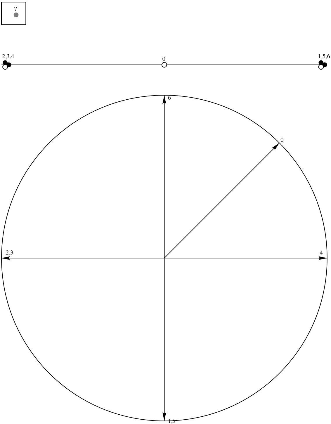
> print $P_I->AMBIENT_DIM, " ", $P_I->DIM;
6 6
> print $P_I->F_VECTOR;
10 39 78 86 51 14
> print $P_I->FACET_SIZES;
8 8 6 6 8 8 8 6 6 6 6 8 6 6
> $facet0=facet($P_I,0);
> print $facet0->AMBIENT_DIM, " ", $facet0->DIM;
6 5
> print rows_labeled($facet0->VERTICES_IN_FACETS);
0:0 2 3 4 5 7
1:3 4 5 6 7
2:2 4 5 6 7
3:0 1 3 5 6 7
4:0 1 2 5 6 7
5:0 1 2 3 4 7
6:1 3 4 6 7
7:1 2 4 6 7
8:0 1 2 3 4 5 6
> $facet0->GALE;
The Gale diagram of facet0 is depicted on the right.